Base class for Electrostatic Solver. More...
#include <ElectrostaticSolver.H>
Public Member Functions | |
| ElectrostaticSolver ()=default | |
| ElectrostaticSolver (int nlevs_max) | |
| virtual | ~ElectrostaticSolver () |
| ElectrostaticSolver (const ElectrostaticSolver &)=delete | |
| ElectrostaticSolver & | operator= (const ElectrostaticSolver &)=delete |
| ElectrostaticSolver (ElectrostaticSolver &&)=delete | |
| ElectrostaticSolver & | operator= (ElectrostaticSolver &&)=delete |
| void | ReadParameters () |
| virtual void | InitData () |
| virtual void | ComputeSpaceChargeField (ablastr::fields::MultiFabRegister &fields, MultiParticleContainer &mpc, MultiFluidContainer *mfl, int max_level)=0 |
| Computes charge density, rho, and solves Poisson's equation to obtain the associated electrostatic potential, phi. Using the electrostatic potential, the electric field is computed in lab frame, and if relativistic, then the electric and magnetic fields are computed using potential, phi, and velocity of source for potential, beta. This function must be defined in the derived classes. | |
| void | setPhiBC (ablastr::fields::MultiLevelScalarField const &phi, amrex::Real t) const |
| Set Dirichlet boundary conditions for the electrostatic solver. The given potential's values are fixed on the boundaries of the given dimension according to the desired values from the simulation input file, boundary.potential_lo and boundary.potential_hi. | |
| void | computePhi (ablastr::fields::MultiLevelScalarField const &rho, ablastr::fields::MultiLevelScalarField const &phi, std::array< amrex::Real, 3 > beta, amrex::Real required_precision, amrex::Real absolute_tolerance, int max_iters, int verbosity, bool is_igf_2d_slices, std::optional< ablastr::fields::MultiLevelVectorField > efield=std::nullopt) const |
| void | computeE (ablastr::fields::MultiLevelVectorField const &E, ablastr::fields::MultiLevelScalarField const &phi, std::array< amrex::Real, 3 > beta) const |
Compute the electric field that corresponds to phi, and add it to the set of MultiFab E. The electric field is calculated by assuming that the source that produces the phi potential is moving with a constant speed  | |
| void | computeB (ablastr::fields::MultiLevelVectorField const &B, ablastr::fields::MultiLevelScalarField const &phi, std::array< amrex::Real, 3 > beta) const |
Compute the magnetic field that corresponds to phi, and add it to the set of MultiFab B. The magnetic field is calculated by assuming that the source that produces the phi potential is moving with a constant speed | |
Public Attributes | |
| int | num_levels |
| std::unique_ptr< PoissonBoundaryHandler > | m_poisson_boundary_handler |
| amrex::Real | self_fields_required_precision = 1e-11 |
| amrex::Real | self_fields_absolute_tolerance = 0.0 |
| int | self_fields_max_iters = 200 |
| int | self_fields_verbosity = 2 |
| bool | is_igf_2d_slices = false |
Detailed Description
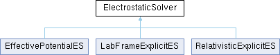
Base class for Electrostatic Solver.
Constructor & Destructor Documentation
◆ ElectrostaticSolver() [1/4]
|
default |
◆ ElectrostaticSolver() [2/4]
| ElectrostaticSolver::ElectrostaticSolver | ( | int | nlevs_max | ) |
◆ ~ElectrostaticSolver()
|
virtualdefault |
◆ ElectrostaticSolver() [3/4]
|
delete |
◆ ElectrostaticSolver() [4/4]
|
delete |
Member Function Documentation
◆ computeB()
| void ElectrostaticSolver::computeB | ( | ablastr::fields::MultiLevelVectorField const & | B, |
| ablastr::fields::MultiLevelScalarField const & | phi, | ||
| std::array< amrex::Real, 3 > | beta ) const |
Compute the magnetic field that corresponds to phi, and add it to the set of MultiFab B. The magnetic field is calculated by assuming that the source that produces the phi potential is moving with a constant speed
![\[ \vec{B} = -\frac{1}{c}\vec{\beta}\times\vec{\nabla}\phi
*\]](form_10_dark.png)
(this represents the term 
- Parameters
-
[in,out] B Electric field on the grid [in] phi The potential from which to compute the electric field [in] beta Represents the velocity of the source of phi
◆ computeE()
| void ElectrostaticSolver::computeE | ( | ablastr::fields::MultiLevelVectorField const & | E, |
| ablastr::fields::MultiLevelScalarField const & | phi, | ||
| std::array< amrex::Real, 3 > | beta ) const |
Compute the electric field that corresponds to phi, and add it to the set of MultiFab E. The electric field is calculated by assuming that the source that produces the phi potential is moving with a constant speed
![\[ \vec{E} = -\vec{\nabla}\phi + \vec{\beta}(\vec{\beta} \cdot \vec{\nabla}\phi)
\]](form_8_dark.png)
(where the second term represent the term 
- Parameters
-
[in,out] E Electric field on the grid [in] phi The potential from which to compute the electric field [in] beta Represents the velocity of the source of phi
◆ computePhi()
| void ElectrostaticSolver::computePhi | ( | ablastr::fields::MultiLevelScalarField const & | rho, |
| ablastr::fields::MultiLevelScalarField const & | phi, | ||
| std::array< amrex::Real, 3 > | beta, | ||
| amrex::Real | required_precision, | ||
| amrex::Real | absolute_tolerance, | ||
| int | max_iters, | ||
| int | verbosity, | ||
| bool | is_igf_2d_slices, | ||
| std::optional< ablastr::fields::MultiLevelVectorField > | efield = std::nullopt ) const |
Compute the potential phi by solving the Poisson equation with rho as a source, assuming that the source moves at a constant speed
![\[ \vec{\nabla}^2 r \phi - (\vec{\beta}\cdot\vec{\nabla})^2 r \phi = -\frac{r \rho}{\epsilon_0}
\]](form_7_dark.png)
- Parameters
-
[in] rho The charge density for a given species (relativistic solver) or total charge density (labframe solver) [out] phi The potential to be computed by this function [in] beta Represents the velocity of the source of phi[in] required_precision The relative convergence threshold for the MLMG solver [in] absolute_tolerance The absolute convergence threshold for the MLMG solver [in] max_iters The maximum number of iterations allowed for the MLMG solver [in] verbosity The verbosity setting for the MLMG solver [in] is_igf_2d_slices boolean to select between fully 3D Poisson solver and quasi-3D, i.e. one 2D Poisson solve on every z slice (default: false) [out] efield The electric field corresponding to the calculated phi (only used with embedded boundaries)
◆ ComputeSpaceChargeField()
|
pure virtual |
Computes charge density, rho, and solves Poisson's equation to obtain the associated electrostatic potential, phi. Using the electrostatic potential, the electric field is computed in lab frame, and if relativistic, then the electric and magnetic fields are computed using potential, phi, and velocity of source for potential, beta. This function must be defined in the derived classes.
Implemented in EffectivePotentialES, LabFrameExplicitES, and RelativisticExplicitES.
◆ InitData()
|
inlinevirtual |
Reimplemented in EffectivePotentialES, LabFrameExplicitES, and RelativisticExplicitES.
◆ operator=() [1/2]
|
delete |
◆ operator=() [2/2]
|
delete |
◆ ReadParameters()
| void ElectrostaticSolver::ReadParameters | ( | ) |
◆ setPhiBC()
| void ElectrostaticSolver::setPhiBC | ( | ablastr::fields::MultiLevelScalarField const & | phi, |
| amrex::Real | t ) const |
Set Dirichlet boundary conditions for the electrostatic solver. The given potential's values are fixed on the boundaries of the given dimension according to the desired values from the simulation input file, boundary.potential_lo and boundary.potential_hi.
- Parameters
-
[in,out] phi The electrostatic potential [in] t current time
Member Data Documentation
◆ is_igf_2d_slices
| bool ElectrostaticSolver::is_igf_2d_slices = false |
Parameters for FFT Poisson solver aka IGF
◆ m_poisson_boundary_handler
| std::unique_ptr<PoissonBoundaryHandler> ElectrostaticSolver::m_poisson_boundary_handler |
Boundary handler object to set potential for EB and on the domain boundary
◆ num_levels
| int ElectrostaticSolver::num_levels |
Maximum levels for the electrostatic solver grid
◆ self_fields_absolute_tolerance
| amrex::Real ElectrostaticSolver::self_fields_absolute_tolerance = 0.0 |
◆ self_fields_max_iters
| int ElectrostaticSolver::self_fields_max_iters = 200 |
Limit on number of MLMG iterations
◆ self_fields_required_precision
| amrex::Real ElectrostaticSolver::self_fields_required_precision = 1e-11 |
Parameters for MLMG Poisson solve
◆ self_fields_verbosity
| int ElectrostaticSolver::self_fields_verbosity = 2 |
Verbosity for the MLMG solver. 0 : no verbosity 1 : timing and convergence at the end of MLMG 2 : convergence progress at every MLMG iteration
The documentation for this class was generated from the following files:
- /home/docs/checkouts/readthedocs.org/user_builds/warpx/checkouts/6102/Source/FieldSolver/ElectrostaticSolvers/ElectrostaticSolver.H
- /home/docs/checkouts/readthedocs.org/user_builds/warpx/checkouts/6102/Source/FieldSolver/ElectrostaticSolvers/ElectrostaticSolver.cpp
Generated by